Today it is already evident that the future is in quantum computing. Quantum computers demonstrate the potential to take humanity to a new level of life.
It is first worth recalling quantum theory to talk about this more substantively. Many people don’t like complicated mathematical calculations, but you can’t perform them without this base. Quantum and classical operations are different. To compare them, there will be shown examples of solving classical problems on traditional and quantum computers in this article. Also, it will be touched on quantum calculus from the application side. You will find an overview of frameworks and cloud platforms for running code and break down a real-world example of a quantum instance.
The Quantum World Is Already Near Us
It may seem to some that quantum computers and everything related to them are somewhere far away and not soon, something from science fiction movies, but it is not so. The quantum world has been around for a long time. And it’s not just about theoretical research. Quantum computing is becoming increasingly popular in business, security, and other spheres.
For example, automaker Hyundai Motor Company and IonQ have announced a new project in the field of quantum machine learning. The idea is that the system will improve skills in recognizing road signs and 3D objects on the road. Thanks to the speed of such calculations, it will come in handy for autonomous vehicles.
Another example is the signing of an agreement between Boehringer Ingelheim, the world’s largest private pharmaceutical company, and Google’s Quantum AI division. The teams plan to create an R&D center to model molecular dynamics using quantum calculus. This will make it possible to speed up and optimize the launch of new drugs on the market. In the same year, NATO said it was testing defenses against cyberattacks using quantum computing. According to the researchers, such computers will be able to find keys to standard data encryption methods quickly. Therefore, today it is necessary to look for new variants to counter hackers.
According to the forecast of the international think tank IDC, the global market for quantum computing will continue to grow rapidly: from $412 million in 2020 to $8.6 billion in 2027. That is, the increase in spending on quantum computing as a service will be at least 50% annually. The prospects are so impressive that it is worth delving deeper into this topic.
Basic Concepts for Working With a Quantum Calculus
Quantum Advantage
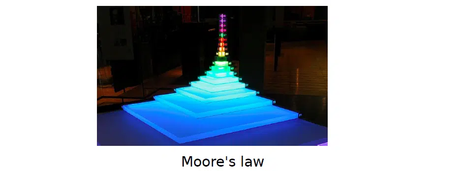
Quantum computers are much more powerful than conventional computers. Suppose you transfer Moore’s law to modern electronics in the form of video cards and central processors. In that case, the technological process of placing transistors on the lining leads to a decrease in the typical package and an increase in the power of computing devices with each period. But in micro- and nanoelectronics, humanity is already approaching transistor sizes of about 2-3 nm. If you go further this way, at this level, the classical laws of physics will stop working, and the rules of quantum mechanics will begin to work.
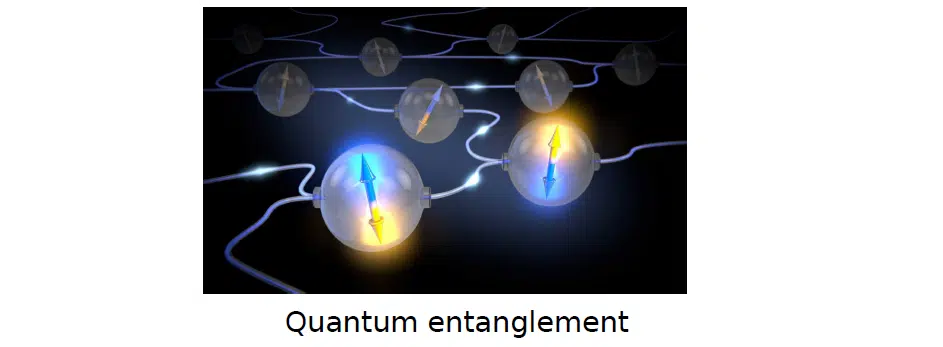
One of the fundamental concepts of this part of physics is quantum entanglement. It suggests that some particles in the quantum world, from electrons to quarks to gluons, can be related to each other. Such particles are called entangled. If you separate them in space and change the spin or orientation of one of them, on the opposite one, the spin of the other entangled particle will change in the same way. This is where the concept of how this can be used from a computational point of view is laid down.
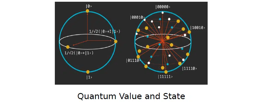
Another fundamental concept is quantum value and quantum state. Let’s break down the meaning and peculiarities of working with them below:
Superposition and quantum uncertainty
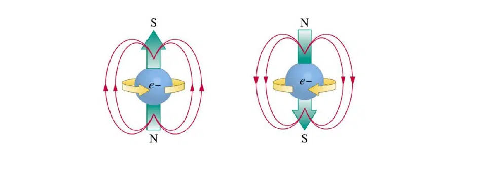
Superposition emerges from the meaning of quantum entanglement. If 2 states are admissible at once in a certain quantum system, then their arbitrary linear combination is admissible too. The main thing to know here is that this law of quantum physics is used for constructing qubits and quantum bits and operations with them.
The principle of superposition manifests itself in many cases, as proven by Schroedinger’s famous cat. This experiment deals with the uncertainty principle. Particles of the quantum world are so small and, at the same time, are in such an enormous volume of space that from the point of view of the deterministic hypothesis, it is impossible to say clearly where one or another of them is located. In other words, each particle is at once at one point and everywhere. Moreover, in the Copenhagen interpretation of corpuscular-wave dualism, a particle can behave both as a particle (i.e., a separate particle) and as a wave. Therefore there are instantiations already built on different principles: wave and particle.
Quantum systems capabilities
Why are quantum computers and systems, in general, quite complex? The problem is not only the size of the particles they operate on. In order to control the quantum world and make measurements more or less accurate, it is necessary to get rid of noise, which appears due to the influence of thermal energy on the quantum system. Because of this, stochastic metrics and probability theory describe the distribution or density of a wave function in a given corridor or some particle. All this is in the process of the quantum computer itself.

The following important concept is stochastic initialization. The system must be initialized before the quantum calculus can be executed. This is done with random numbers, which are later subject to quantum optimization. However, this initialization affects the quantum world and depends on environmental noise. Therefore, there should not be deterministic distributions of metrics but precisely stochastic ones.
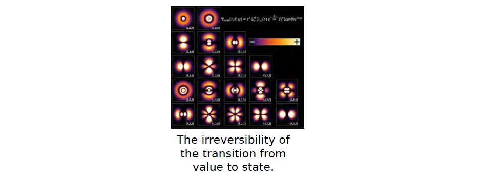
A quantum system cannot go back from a value to a state. First, it is in a state of superposition. But after measuring this state, the system goes to the deterministic order, which is the value already. Therefore, the system cannot return to a state of indeterminacy. This is a very crucial element related to the pretrain of quantum models.
It is also worth remembering the sensitivity to noise. This is one of the biggest enemies, significantly affecting the quantum system’s state. To fight it, developers of quantum computers endow them with a huge refractor, which operates at mega-low temperatures, not to level thermal entropy. Although the CPU itself in quantum technology is relatively small.
Values vs. state
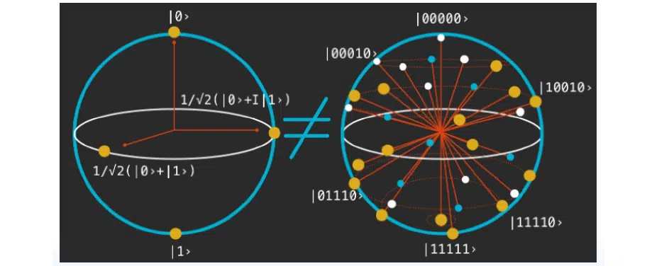
There is no exact understanding of how to do it. This state of the system is exactly what is called a state. And after measuring a qubit or some other particle, you observe, fix, and get values. These concepts should not be confused, because they are irreversible. On the left side of the picture are concrete values—fixed qubits on some bases. They cannot be returned to a random stochastic interpretation of the quantum system, as shown on the right:
Examples of Classical Tasks
MNIST Classification
How about solving a well-known problem among data scientists, the MNIST Classification problem? It has a dataset of handwritten digits with several classes from 0 to 9.
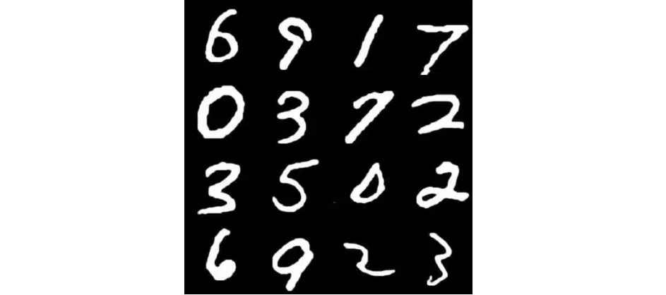
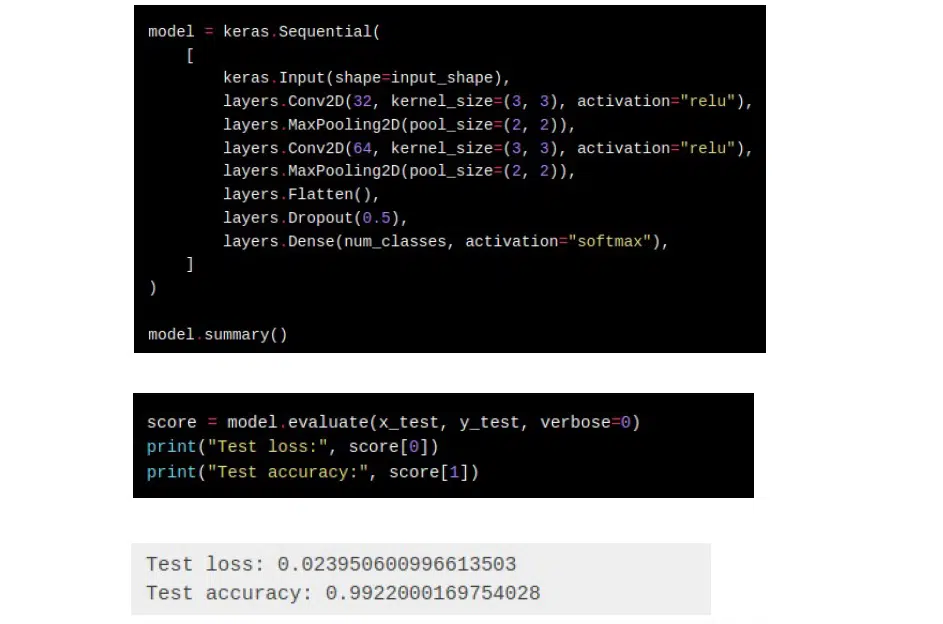
A simple model to solve this problem is needed, assembled in the code below. There are some input and convolutional burns, and the classification goes simply to softmax. The accuracy of such a dataset is very high—in our case, 99.22%. A few epochs are needed to achieve the static power of the system.
In the usual interpretation, it all works clearly. The model, outputs and inputs, layers, all mathematics, and even data are represented as a binary interpretation. Everything is encoded in the traditional sequence of zeros and ones.
Quantum systems
To understand how to solve such a problem with a quantum system, it’s necessary first to understand what qubit and bracket notation, also known as Dirac notation, are from a mathematical point of view.
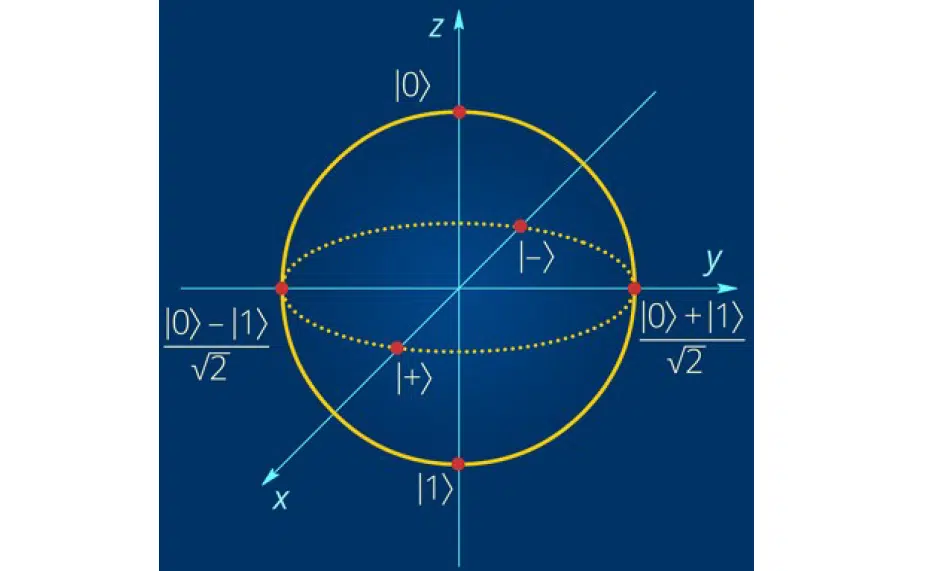
The illustration shows the classical bit and the quantum interpretation applied to Bloch’s sphere:
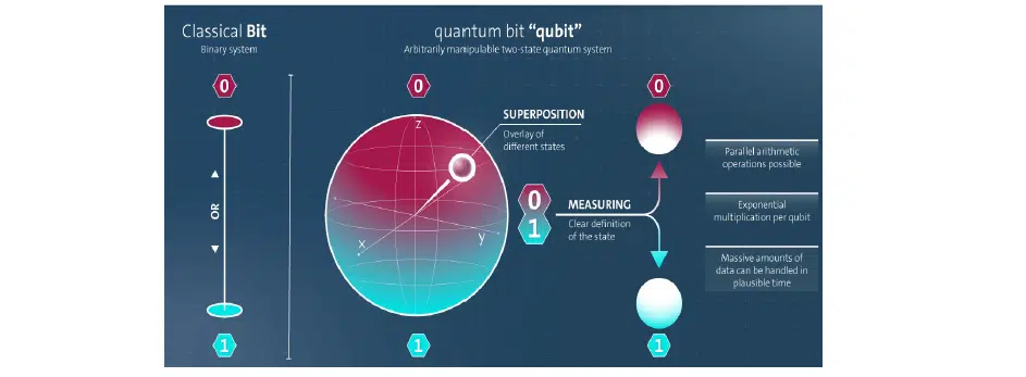
A qubit is a vector of complex digits. The vast majority of quantum systems or computers are based on lasers. To operate them, it is necessary to control the amplitude-phase partial characteristics, which are very well described by complex numbers. Therefore, when Niels Bohr was confirming the various hypotheses of quantum mechanics, these mathematical tools were already quite well known. Because of this, the complex-valued interpretation significantly simplifies the mathematical calculations.
The generalized form of quantum bit is written as shown in the left part of this expression:
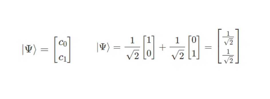
If you need a qubit of this form laid out on the basis, you should apply the formula as given on the right. It all looks pretty simple, just like in linear algebra. However, there are no complex-valued numbers in this example; they will be addressed in the next subtopic.
Quantum bases and Bloch’s sphere
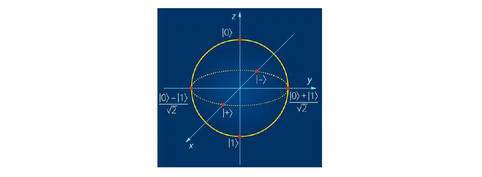
In classical quantum mechanics, there are several essential bases: Z-basis, Y-basis, and X-basis. For quantum calculations, Z-basis is used. It is closer to the perception by Data Scientists and scientists who have worked on optimization problems or with classical machine learning. When making measurements on the Bloch sphere, it will be easier to interpret qubit values that are closer to 1 or 0 than to some complex-valued numbers. Although, this does not rule out the possibility of using Y- or X-bases. In some cases, their use is more convenient.
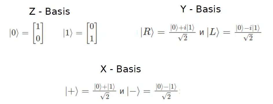
As for the Bloch sphere, it is just some interpretation of the distribution of qubits in space. Basis minus and plus, denoted as X, are directed along the X-axis, Y-basis—Y-axis, and Z-basis—according to the Z-axis.
Quantum gates and rotations
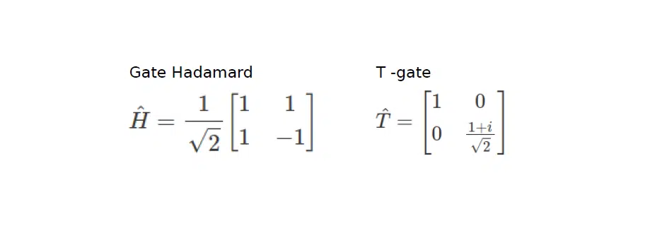
When you deconstruct qubits as complex-valued numbers on some bases, the question arises: what do you do with them next? To carry out optimization, some parameters of the quantum system are necessary. That’s where quantum gates—operators based on which more complicated quantum circuits are built—come in handy. The most common operators are Adamar’s gate and T-gate. According to the entrepot sequence theorem of quantum schemes, any complex quantum system can be reduced to a sequence of precisely these gates.
Also famous is the CNOT gate, which inverts one observer bit and one control bit. The diagram below shows how to initialize a quantum circuit with this operator:
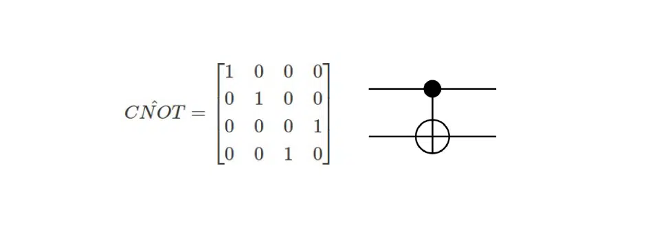
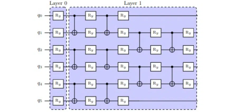
These operators allow the building of quantum circuits. The expression below shows how to obtain from basis 1 0 the qubit considered above. To do this, one must multiply the Adamar operator, which represents some tensor, by a column vector, and obtain the value of the vector:
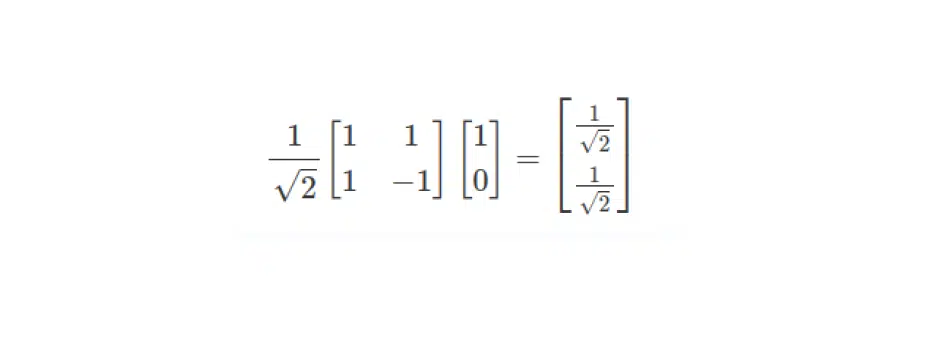
It is not enough to set bits and pieces and figure out how quantum circuits are prepared. To move from the quantum system’s entangled value and perform the measurement, it is necessary to set Pauli operators (operators of measurement). You can read about them in more detail in any quantum theory. But let’s limit to the fact that Pauli operators are the basic concept in obtaining or transferring the quantum system from superposition state to value state.
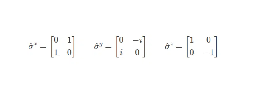
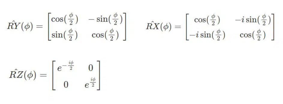
To change the qubit’s value, it should be rotated around the Bloch sphere. Therefore, it is worth considering the operators RY, RX, and RZ. Again, if you wish, you can read this theory on your own.
In the already-mentioned scheme, the qubit q0 is initialized and twisted around the RY axis, i.e., multiply by the RY matrix. This will allow it to change values on the Bloch sphere:
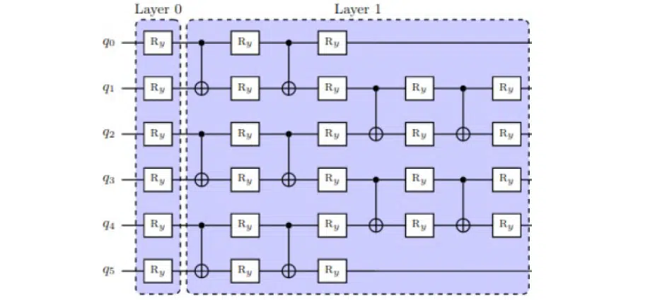
Why exactly is rotation a key to finding the optimal value of the state of a quantum system? When rotating qubits, they will change their values. If you construct a closed loop of optimization, it is possible to understand which value of this particle will make the quantum circuit most effective in solving the task:
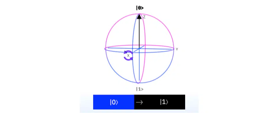
But you have to be careful here. If you initiate and twist around the RX axis, the Pauli operator must measure the values of the particles on the Z-axis. Why? If you twist the initialized zeros, then the value of Z changes completely, from null to first. If, on the other hand, one twists around the Z-axis and measures with the operator Σ Z, then the value of Z is unchanged. This may greet the quantum embedding of the data in the general model. Instead of a variational scheme you will get garbage from the data.
Quantum Calculus in Machine Learning
Finally, let’s look at calculus techniques and figure out what to do with translating classical data into the quantum world.
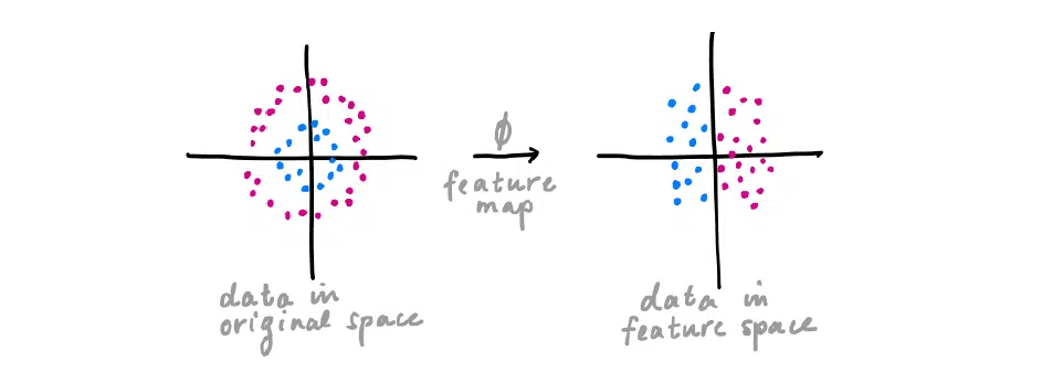
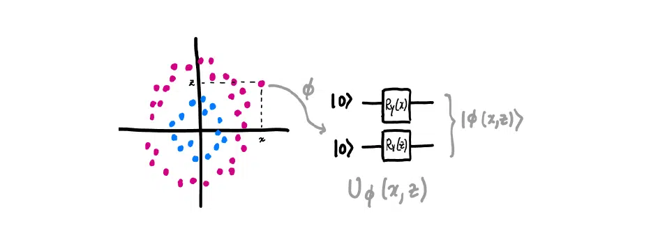
There are some classical data in some space. When you build a machine learning model, you will actually get a feature map—a certain imbanding with well-distributed data in another space. That’s what this model is built on:
But in the quantum world, the data must be encoded before it can be applied. The following shows how one can encode some data points in a certain generalized space. A bit is used to initialize each data point. It can be not only 0. Then there is a rotation, due to which each data point is encoded in some form and goes to quantum optimization:
Quantum gradient
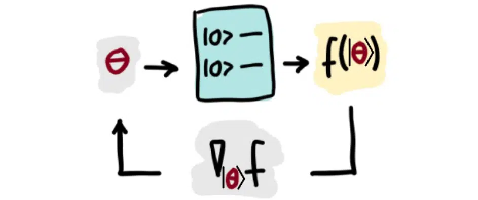
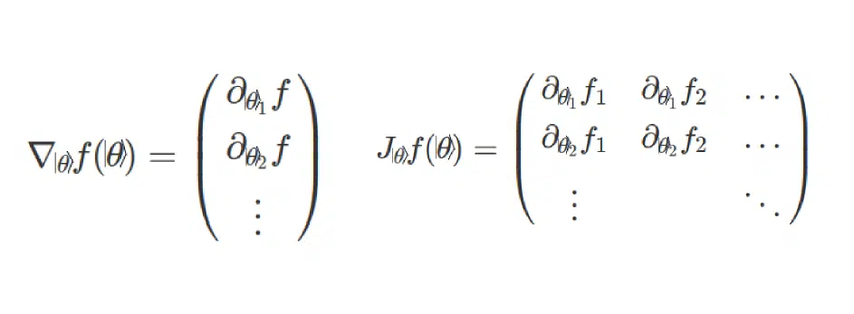
To do quantum optimization, you also need to understand how close you are to the optimum of the target function. It is written in classical machine learning with a loss function. The illustration below shows a diagram of this process. Classical data is encoded to the quantum type, and the loss function is found, followed by the gradient or Nabla operator. If there are many layers, you get a Jacobian matrix. The result is that everything gets looped and repeats round after round:
As for the formulaic form, this process is described as follows:
Types of calculus:
- Classical calculus. All data, models, inputs, layers, instances, and others are represented in classical form.
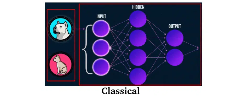
- Combined methods. This is a combination of the two worlds. For example, the data is encoded in quantum form, and for the solution apply the classical model (as in the first scheme). Because of the influence on quantum mechanics of thermal entropy, there are often problems with finding quantum gradients. Therefore a combination of quantum and classical calculators is used. Sometimes there is an inverse combination: data is in a classical form, and the model is a quantum interpretation (the second scheme).
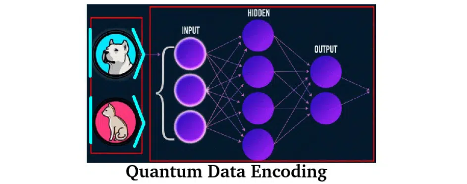
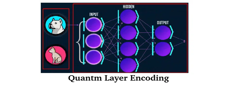
- Completely quantum calculus. Both data and itself are model-encoded in quantum form. This scheme is the most promising.
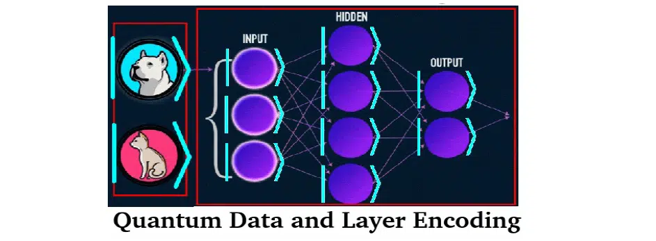
Frameworks and Сloud-based Quantum Instances
Quantum mechanics and calculus are already so common that there is a reasonably wide range of programming languages. For example, Q# from Microsoft, PyQuil, Qiskit from IBM, and Pennylane. Let’s consider the last one.
It is worth noting that there is no such thing as quantum machine learning when solving quantum problems. There is quantum optimization, optimization of quantum schemes. Machine learning can be tied to this process, since ML is essentially optimization. Pennylane is a convenient and, most importantly, cross-platform tool. But Q#, PyQuil, and Qiskit work only on Microsoft and IBM solutions, respectively.
As for the service, let’s talk about AWS Bracket, where you can run IBM and Microsoft Quantum. It provides quite a high variability of quantum calculators. Their choice is also relatively wide. You can think of D-Wave, IonQ, Rigetti, and OCQ. Let’s pay attention to the first two because they are the most popular on the market right now.
What it looks like on a real quantum instance
To assess the capabilities of these instances and work with them, let’s take MNIST Classification, QNN, as an example, and present a 28×28 image. Encode each pixel with a quantum scheme. First of all, initialize it with zero qubits. To be emphasized: these are not streets, but kills—that is, in expanded form 1 0 1 0 0 1 0. In this way, go through with a one-pixel offset across the entire image. This is what quantum layout is when a quantum G circuit is constructed and a measurement is made for each channel.
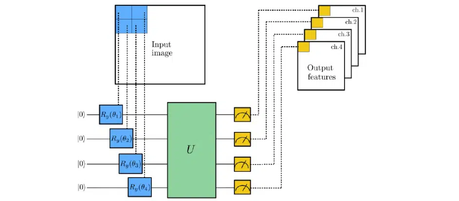
At the code level, it looks like this. The first step is to install the Pennylane library, then import RandomLayers, which will initialize the quantum layouts, and NumPy, which is imported from the Pennylane library and supports quantum tensor operations.
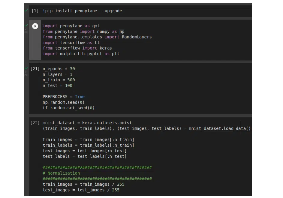
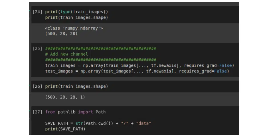
To show the fundamental difference, let’s use 500 samples for the train, 100 samples for the test, and 30 samples for epochs. One layer also will be taken and run on a simulator when the quantum schemes are simulated with a classical CPU. You can see how long it takes so you can compare it with quantum instances later. The process itself is uncomplicated: first, there is a simple split operation, then the data is normalized and stored, and when it is finished, it creates parsing for the channel.
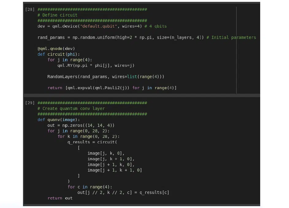
The most interesting things happen in the following blocks of code. The first is the creation of a quantum socket or quantum circuit. The second is the creation of the quantum layout. In this case, 4 qubits are taken, choose the default qubit as a device and initialize with random parameters. The angle can be anything— for example, chose 2 multiplied by pi. It is not important, because in the process of optimization the angle will change. To build a socket, you need to turn the function into the qnode decorator from the Pennylane library. Note that here the rotation is done around the y-axis. Then throw the parameter into RandomLayers and measure around the Z-axis with the Pauli operator. This is a crucial aspect. But the quantum layout is simple: from an image of 28×28 you get the next layout already in the form of 14×14. It should be done for each pixel and return the result.
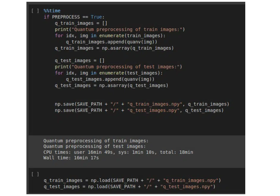
Next, let’s put everything to work. It took about 18 minutes on a conventional CPU.
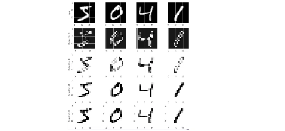
If you plot this image, there is some variation behind the channels. channels 1, 2, and 3 are very different, and only channel 5 more or less resembles the previous one. However, this is not a problem. You just need to be aware of this effect.
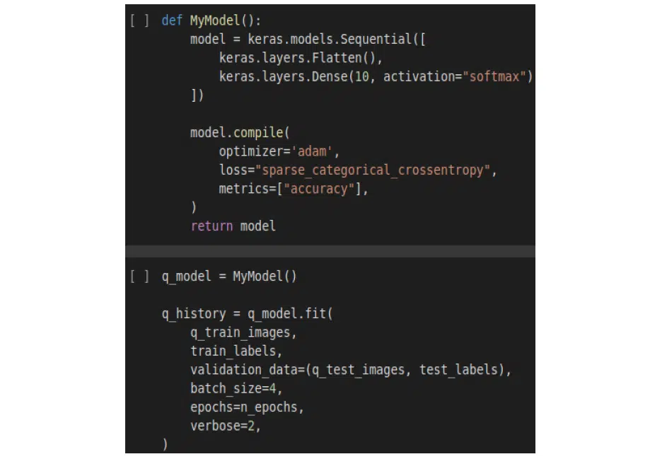
Now train the softmax model with the parameters shown in the illustration. These are categorical cross-entropy and accuracy metrics:
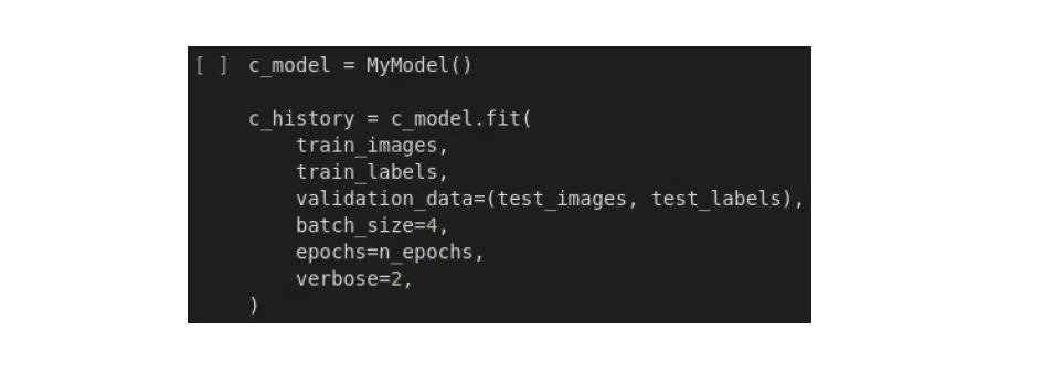
Also, train the classic model:
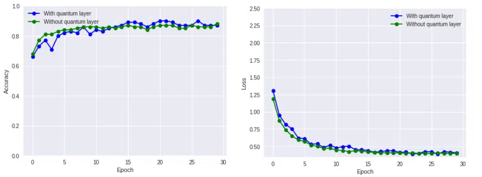
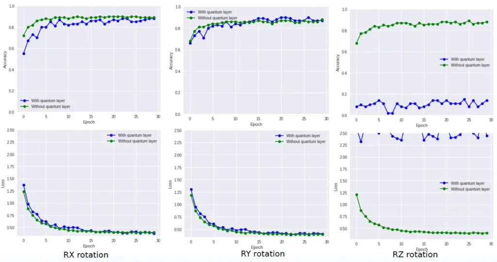
Below you can see that the accuracy is almost the same, but below the mentioned 99.22%. To remind you, it’s taken a significantly smaller number of samples. The main thing is that here you can perfectly see the characteristics of the quantum system. It looks like a fence due to the simulated noise, but without the quantum layer, it is smoother:
Next question: what is the effect of the rotation itself? Let’s keep the system configuration in the previous form and rotate qubits in different directions. The results are in the next illustration. RY you have already seen above, on RX the picture is similar, but with RZ all is bad, since here the previously mentioned quantum entanglement is observed:
Let’s consider this situation in more detail. If you look at the resulting images, you can see that channels 2, 3, and 4 are almost identical (channel 5 wasn’t output).
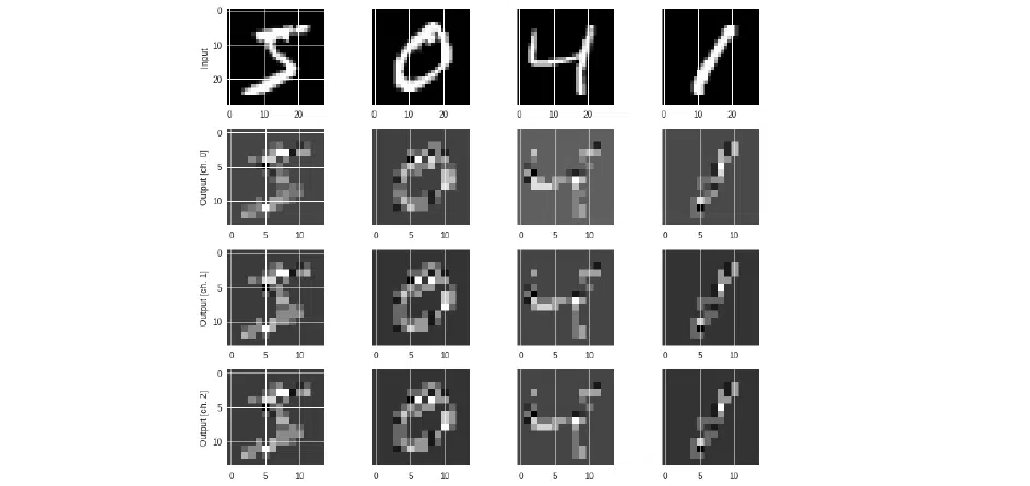
That is, if you rotate around the Z axis a qubit that is directed in a certain way on the Block sphere, then the Z of that particle does not change. Although, when measuring X and Y, the variation of different channels does not disappear anywhere. This is a big mistake, it should be monitored carefully.
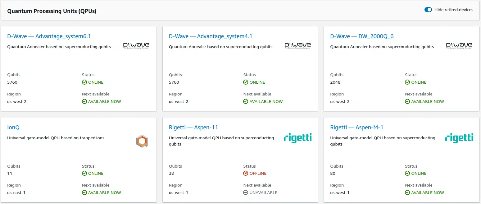
AWS offers quite a few quantum calculators to solve the problem. You have a choice of instances of D-Wave, IonQ, and others. Let’s choose D-Wave for 2048 qubits and IonQ for 11 qubits. By these metrics, the former seems much more powerful. However, in reality, the situation is not so straightforward. The D-Wave by its quantum-physical nature works exactly with wave functions. This is the crudest interpretation one can have. IonQ works with full-fledged qubits. And while D-Wave needs several wave functions to implement a qubit, IonQ has exactly one qubit responsible for the qubit. When comparing the power of these instances in the same tasks, the difference is hardly noticeable. Although due to the possibility of complex implementation of more full-featured qubits, D-Wave can sometimes win.
Running on a Real Instance
When comparing the diagrams below, you can see a fundamental difference between the two models. The classical approach deals with neurons, activation functions, SPG propagation, gradients, etc. However, in the quantum system, there are no neurons. Here is built a sequence of sockets in a certain way and tried optimization of them through rotation to obtain a qubit in the space that would be able to solve the problem as accurately as possible. To simplify things a lot, this is what a neural network on a quantum calculator looks like compared to a conventional one:
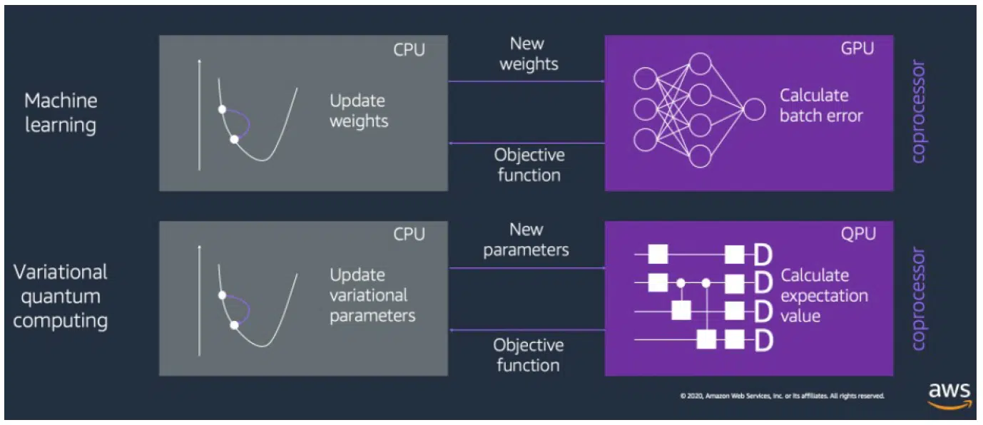
You should also remember that IonQ has topology: its 11 qubits are connected and entangled one by one. D-Wave has no such thing since it works with wave function operators, and the qubits are incomplete. Because of this, physically, the principle of the calculus of these systems is fundamentally different, but in practice and for us, there is no difference. To run a Pennylane task on an AWS instance, you need to register the selected instance and pass the endpoint to Pennylane, which only requires you to join. The framework itself does the computational math. All we have to do is build the quantum optimizer.

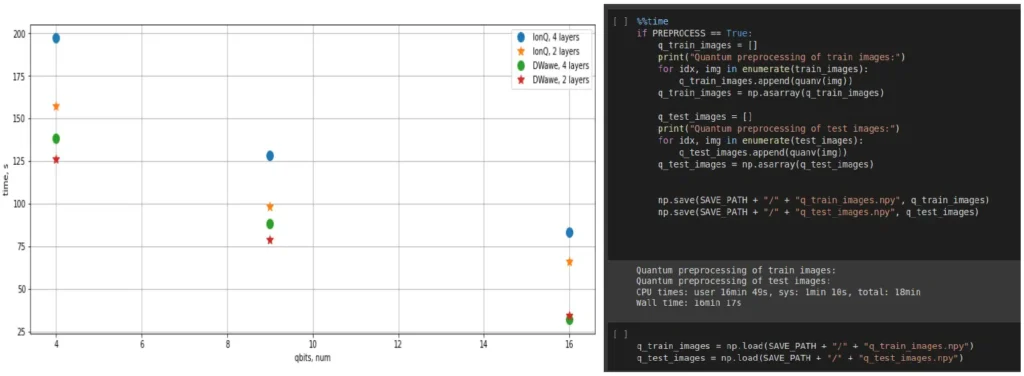
There was used IonQ of 2 and 4 layers to calculate the example and D-Wave of 2 and 4 layers. 4, 8, and 16 qubits were used for each layout to look at the results. They are not significantly different from each other in terms of the computational power of quantum instances. However, they are very much better than the conventional CPU.
Below the screenshot with the past results on the classical computer has been repeated, where the process lasted about 18 minutes. IonQ for 4 layers reached the same result in about 200 seconds (for 2 layers even less). In D-Wave, the results are even better. A savings of about 6 times—that’s very cool. By the way, the dependence may seem linear, but it is quasi-linear.
You may have a question: won’t the performance be even better with GPUs? Truth be told, these devices are faster, but only at this time. In the future, they will definitely lose to quantum computers.
Let’s summarize the most important things:
- Basic optimization of quantum schemes is the rotation itself. To obtain optimum quantum system values, one only has to rotate qubits, which will be based on a quantum gradient.
- Choice of a correct rotational direction is a fundamental concept of performing quality quantum optimization.
- Quantum computers allow people to solve existing problems and train ML models. But it is necessary to see the future. Although a GPU allows experts to solve a wide range of problems, in about 10 years, there will be complex models which require a fundamentally different approach. And here, quantum computers themselves will be of use for business.
- Quantum pretrain is impossible, and this is sad. Typically, pretrain consists of training the model, saving the value, and using the physical model to obtain new results. The quantum model has a different principle: when it is exercised, values are not taken off. Because they are in the superposition state at the moment of signal passing. This is the reason why everything works very quickly and one-time. If the value is removed, all magic of the quantum system collapses. That is why for this purpose, probably, it is necessary to look for other approaches.
- Quantum calculations are still influential in comparison with classical approaches and pipelines. Today there are a lot of traditional pretreatment models and ready implementations which can be found on the tensorhub. You just need to convert the required one, modify it to your conditions and start production. With quantum models, it is still tricky. Moreover, you cannot put a quantum computer under the table and have to turn to cloud instances, which are expensive nowadays, and it is essential to scale them.
Quantum computers will be the main reason for the emergence of the first human-like piece of artificial intellect. Such a development will be trained and make crucial decisions. At the same time, it will do everything on one domain. A quantum system will be able to synthesize data from different experiences and get fundamentally new conclusions compared to modern models. So the world is on the threshold of a real revolution, and you, as data scientists, can already reach it.
